On sharks and ice creams
Again this year I am teaching a part of the PAMI class at Politecnico di Milano, Como campus. My personal objective in this class is not just to teach students how to use a tool (R) to perform statistical learning, but also to give them the confidence they need to use R and assess their own knowledge of the topic by playing with exercises and experiments (see e.g. the homeworks I published last year).
For this reason, I usually take some pretty well-known problems and try to explain them while modeling them in R. In the process I show what kind of out-of-the-box commands can be used to solve these problems, but also how to obtain the same results step-by-step, creating a link between the equations in their textbook and the R code they write.
Last week I gathered some material to explain that correlation does not imply causation. The first thing that struck my interest is that you can find pretty funny visual examples online, amongst which the ones I liked most are XKCD’s:
and Adam Sandiford’s one:

Then I googled the pretty popular sharks and ice creams example and I was amazed to find a lot of material: books, news articles, sci-fi tales, and of course reddit posts. And I almost forgot, there also is Jaws Bar, one of the top 10 Korean ice cream bars according to The Korea Blog:

As you might guess, this was not exactly the kind of answer I wanted for my class. Surprisingly (or maybe not so), the most pertinent material I found comes from college-level AP Statistics (see e.g. here). The most interesting hint I found was in the article Bundled-Up Babies and Dangerous Ice Cream: Correlation Puzzlers (which, of course, I could not download despite working in a university: thank you JSTOR). The idea of encouraging students to think critically about correlation by letting them discover lurking variables was exactly what I wanted to put in practice, and to do that I decided to actually populate a dataset with ice creams, people eating them, and sharks eating them (the people, not the ice creams… Well, actually both in some cases).
This small tutorial assumes you already know at least the basics of linear regression with R. If you don’t, you can easily catch up by reading the first two chapters of An Introduction to Statistical Learning and checking out my notes (labs 1 to 4) here. Then just fire up R and start creating some observations using the rnorm() function. First people: for 100 days, we count how many people entered a beach and observe 400 on average per day (with some variance, to take into account days with special events or bad weather):
# set the seed to some fixed value so we all have the same results
set.seed(12345)
# 12345? That's amazing, I got the same combination on my luggage!

# let us create our dataset: first people...
people = rnorm(100,400,60)
Then we add both ice creams and sharks. For ice creams, let us say that on average 3 people out of 10 buy one:
# icecreams (we use floor() so the number of sold ice creams is an integer)
icecreams = floor(.3 * people + rnorm(100, 0, 5))
cor(people,icecreams)

# [1] 0.9718321 a pretty high correlation
# let us plot icecreams vs people
plot(people,icecreams)

# fit icecreams sales wrt people
icecreamsFit = lm( icecreams ~ people )
abline(icecreamsFit,col="red")
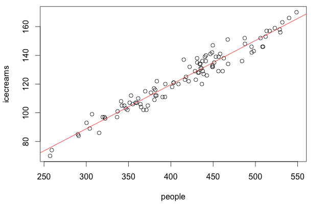
What you see above here is the plot of ice cream sales as a function of the number of people. The R function lm() is used to perform linear regression on the input data (in this case, fitting a linear model which describes icecreams as a function of people). Finally, abline() plots the fitted function that approximates the linear relationship.
Shark sightings can be modeled in different ways: I will choose a very trivial model for explanatory purposes, but the same reasoning can be applied also with a more realistic one. Suppose we have some sensor alerting us whenever a shark enters an area which is close to the beach: the alert can be triggered many times by the same shark, whenever it exits the “safe area” and enters it again. The data we get show a simple linear relationship between shark sightings and the number of people at the beach, e.g. one every 10 people (yes, it is high… this is why, to make it less gory, I wrote shark sightings instead of attacks):
# sharks (one sighting every 10 people)
sharks = floor( 0.1 * people + rnorm(100, 0, 5))
cor(people,sharks)

# [1] 0.8141827 a good correlation between sharks and people too
# let us plot sharks vs people
plot(people,sharks)

# fit sharks sightings wrt people
sharksFit = lm( sharks ~ people)
abline(sharksFit,col="red")
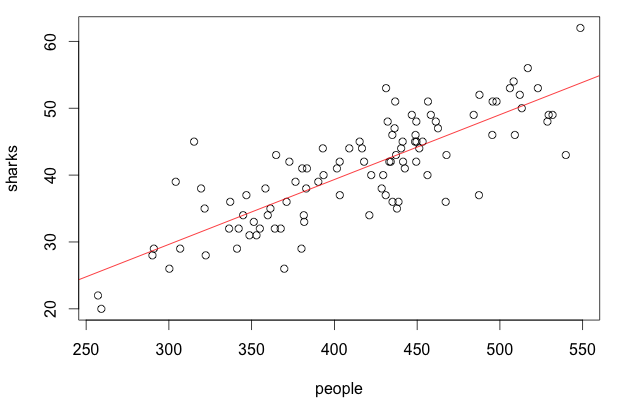
Note that, even in the case of sharks, we floor() the number of sightings to always obtain an integer value. Note that, as a consequence of linear regression, during prediction we might end up with non-integer results whose interpretation is not as intuitive. Let us not worry about this for the sake of this example, and focus on the relationship between the variables we have just created. Here are the results of the summary() command on the two fits:
summary(icecreamsFit)
    Call:
    lm(formula = icecreams ~ people)
    ...
    Coefficients:
                 Estimate Std. Error t value Pr(>|t|)
    (Intercept) -3.313835   3.161898  -1.048    0.297
    people       0.307307   0.007528  40.822   <2e-16 ***


summary(sharksFit)
    Call:
    lm(formula = sharks ~ people)
    ...
    Coefficients:
                Estimate Std. Error t value Pr(>|t|)
    (Intercept) 0.551531   2.933507   0.188    0.851
    people      0.096955   0.006984  13.882   <2e-16 ***
In both cases we were able to fit a model which is pretty close to the actual function we used to generate the data: the slope for the two lines is very similar to the one we set up, and the high p-values for the null hypotheses on the intercept give us a hint that they are likely to be zero and should be taken out of the model (if you want to better understand null hypotheses and p-values, this is a pretty good introductory video). This was expected, as the data we generated has a rather low noise and the correlation between the input and output variables is pretty high.
What about the relationship between sharks and ice creams, then? Let us suppose we do not have access to the people variable, and try to fit a model which describes the number of shark sightings as a function of the ice cream sales:
# now let us see what happens with sharks and ice creams...
plot(icecreams,sharks)
cor(sharks,icecreams)

# [1] 0.7739648 hmmm... This is pretty high too.
# Does this correlation imply causation?
sharksIceFit = lm( sharks ~ icecreams)
abline(sharksIceFit,col="red");
summary(sharksIceFit)
    Call:
    lm(formula = sharks ~ icecreams)
    ...
    Coefficients:
                Estimate Std. Error t value Pr(>|t|)
    (Intercept)  4.58021    3.03281    1.51    0.134
    icecreams    0.29147    0.02409   12.10   <2e-16 ***
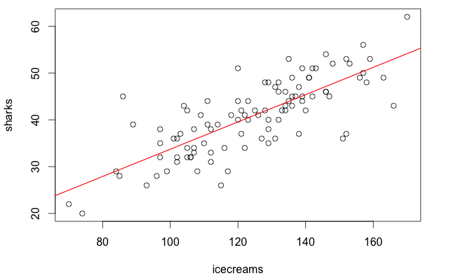
Aaaand here it is: both ice creams and sharks depend on people, but if we take people out of the model it really looks like there is a linear relationship between them! If you just trusted the results of this regression, you would deduce that you can explain an increase in shark sightings with an increase in ice cream sales, basically concluding that ice creams cause sharks to approach… But you know this is plain wrong! How can one be more confident on her own conclusions, then?
The first question you should ask yourself is “did I take all the variables into consideration?”. If the answer is no (likely to be true, if you have considered only one input variable), you should include them in your model too. For instance, if we also had access to the people variable we could use it to run a multiple linear regression:
# let us try multiple linear regression
allFit = lm( sharks ~ people + icecreams )
summary(allFit)
    Call:
    lm(formula = sharks ~ people + icecreams)
    ...
    Coefficients:
                Estimate Std. Error t value Pr(>|t|)
    (Intercept)  0.16318    2.94132   0.055    0.956
    people       0.13297    0.02955   4.500 1.89e-05 ***
    icecreams   -0.11719    0.09345  -1.254    0.213
Note that when you choose to include more variables in your linear model, the results you get from the null hypothesis tell you something different. In simple linear regression, the question you try to answer is whether any change in an input variable causes a change in the output while ignoring all the other variables. In simple words, it would be the same as asking “If sharks sightings did not depend on anything else, would they depend on ice creams sales?”. In multiple linear regression, you want to verify whether changing an input variable affects the output while all of the other variables in the model stay the same. It would thus be the same as asking “If sharks sightings could depend on different factors such as icecreams and people, would they depend on ice creams sales and/or people?”. And the answer, as you know in this case, is that they do not depend on ice creams.
A second question you should ask yourself is “did I take all the variables into consideration?”. Yes, that is the same question as before :-). The reason is that I do not want you to be misled by this simple example: even when you have a model that voids a previous, simpler hypothesis, that does not mean this is the best possible one! Look at this other example:
# we generate 100 temperature values
temperature = rnorm(100,20,5)
people = 10 * temperature + rnorm(100,-50,12)
sharks = floor(0.5 * temperature + rnorm(100, -1, 1))
icecreams = floor(.3 * people + rnorm(100, 3, 5))
Here we suppose that temperature positively influences both the number of people at the beach and the number of sharks that will approach the shore. Ice creams, instead, are modeled as depending on the number of people. If we run the same multiple linear regression as before, this is the result:
allFit = lm( sharks ~ people + icecreams )
summary(allFit)
    Call:
    lm(formula = sharks ~ people + icecreams)
    ...
    Coefficients:
                Estimate Std. Error t value Pr(>|t|)
    (Intercept)  0.65904    0.43566   1.513    0.134
    people       0.04444    0.00731   6.079 2.38e-08 ***
    icecreams    0.02617    0.02378   1.101    0.274
This correctly shows that sharks sightings do not depend on ice cream sales, but does not say anything about the temperature (of course: we did not include it into the model!). And the conclusion looks so similar to the previous one that you might easily mistake people as the real cause for the increment of shark sightings.
On the other hand, if all the variables we defined in our example are correctly taken into account, we can have a good estimate of what causes what:
allFit = lm( sharks ~ temperature + people + icecreams )
summary(allFit)
    Call:
    lm(formula = sharks ~ temperature + people + icecreams)
    ...
    Coefficients:
                Estimate Std. Error t value Pr(>|t|)
    (Intercept) -1.19984    0.71981  -1.667  0.09879 .
    temperature  0.35574    0.11232   3.167  0.00206 **
    people       0.01331    0.01206   1.104  0.27242
    icecreams    0.01325    0.02311   0.573  0.56770
At this point, I think the main question you might have is “how can I be sure, then, that I have taken all of the right variables into account?”. Well, in many cases you cannot really be sure, but asking yourself this question is already a step in the right direction to avoid misinterpreting your data… Which is why I leave you with the following quote from danah boyd’s Six Provocations for Big Data:
Interpretation is at the center of data analysis. Regardless of the size of a data set, it is subject to limitation and bias. Without those biases and limitations being understood and outlined, misinterpretation is the result.